Particles are tiny visual elements. They are useful for creating striking motion. With JavaScript and WebGPU, it is possible to build particle-based visuals on the web as well. Using a text-based effect as the example, this article introduces ideas and implementation details that are useful when creating particle effects.
Demo
Here is the finished result of the tutorial in this article.
What this article covers
- Turning 2D text into particles and animating it
- Using Perlin noise to create a sense of atmosphere
- Managing large numbers of tweens with GSAP
- 2D rendering with WebGPU using PixiJS v8
Technologies used in this demo
This section gives a quick overview of the web technologies used in the demo.
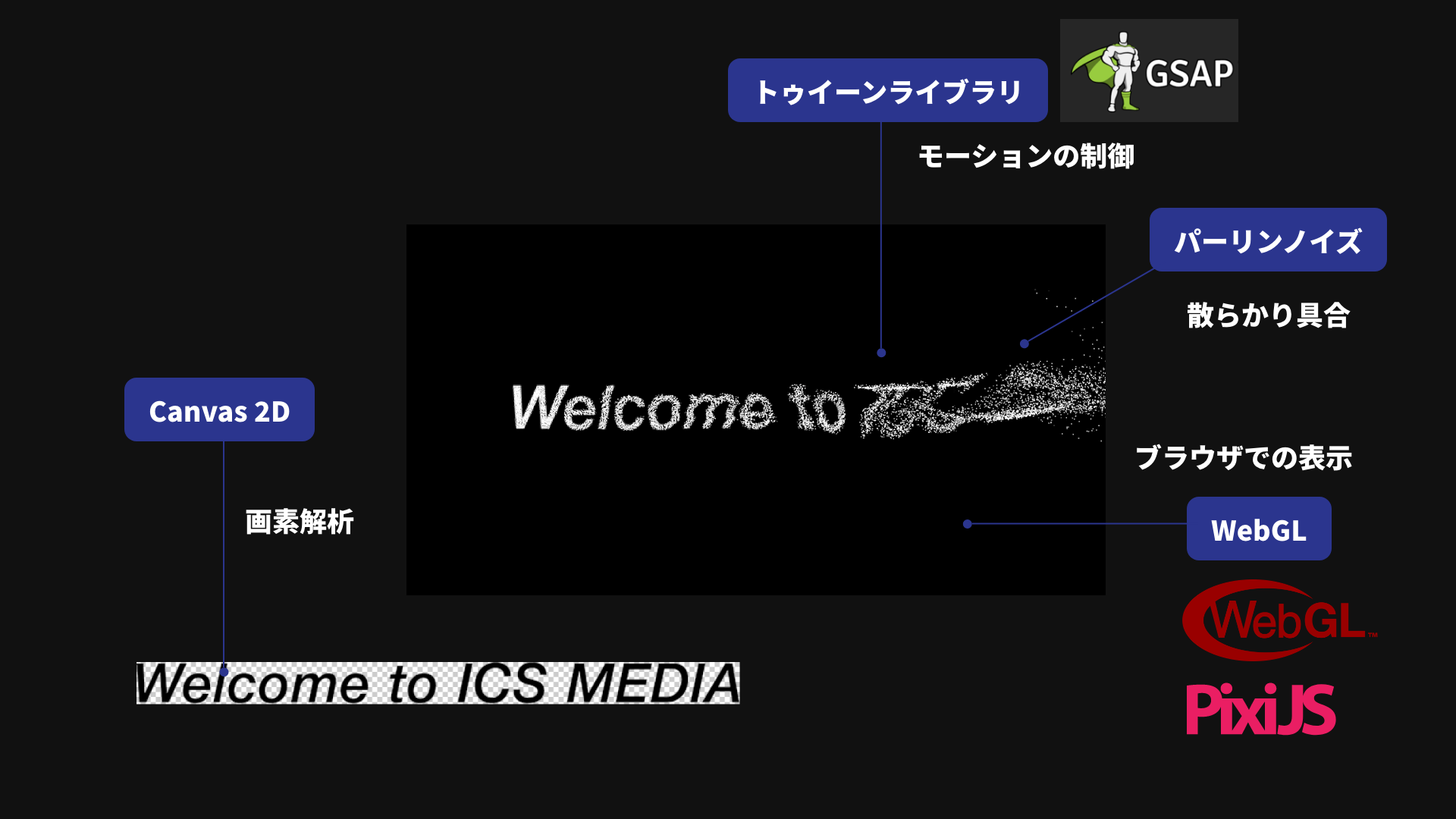
WebGPU
Rendering is handled with WebGPU. In the demo code, preference: "webgpu" is passed to PixiJS v8’s Application.init(), so drawing is done with WebGPU. WebGPU is often thought of as a technology for 3D graphics, but it can be used for 2D as well.
One of the best-known GPU rendering libraries for 2D is PixiJS. It is highly performant and provides an API reminiscent of Adobe Flash. This demo uses PixiJS, but any JavaScript library is fine as long as it can render with WebGPU.
Canvas 2D
Canvas 2D is used to analyze pixel data from the image. This is needed later to determine whether a given pixel is blank.
Tweening
Motion is created by specifying positions at keyframes and interpolating between them. This interpolation technique is called tweening. In this article, tweening is handled with GSAP, a JavaScript library. GSAP is recommended because it performs well when many tweens run at the same time, though other JS libraries would work too.
Deterministic randomness
To generate Perlin noise, we use the JS library josephg/noisejs. Other libraries can also implement Perlin noise, so a different JS library would work as well.
Build it in four steps
We will create the effect with the following approach.
- Draw the text onto a canvas
- Break the text into particles
- Scatter the particles
- Add a wind-like flow to the motion
The idea is to have a large number of particles gather together to form the shape of the text.
Step 1. Draw the text onto a canvas
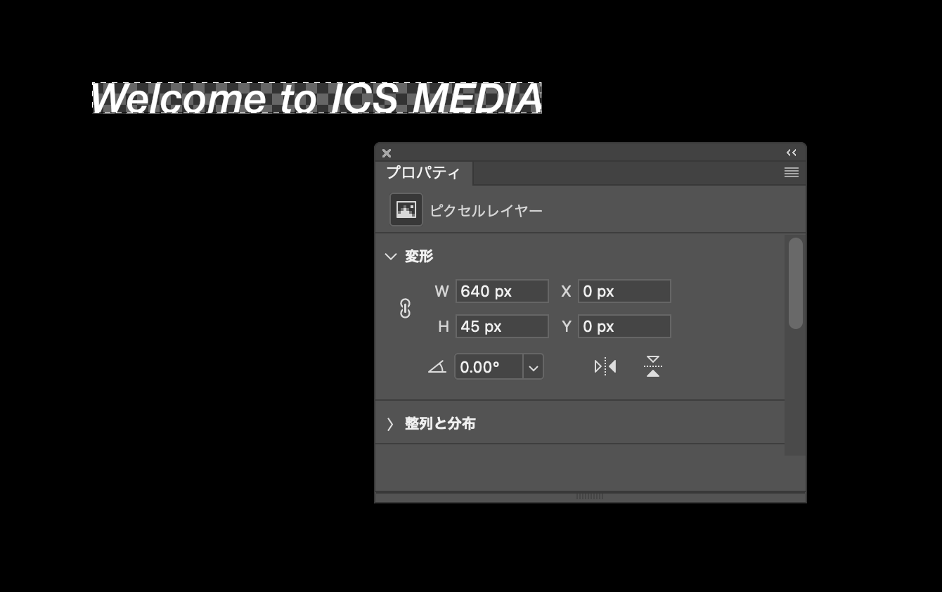
Prepare a transparent PNG image that contains the text.
Load the transparent PNG with JavaScript. Because we want to handle it synchronously, create an Image object and wait for its decode() method with await.
// Load the source text image.
// Later, only the opaque pixels in this image will be converted into particles.
const image = new Image();
image.src = "images/text_2x.png";

// Later steps use the image dimensions and pixel data,
// so wait for decode() to finish before continuing.
await image.decode();
Draw the image into CanvasRenderingContext2D (referred to here as Canvas 2D), the 2D drawing API of the canvas element. Once the image has been copied into Canvas 2D, its pixel data can be inspected.
// Store the image dimensions.
// These are used when sizing the canvas and positioning the particles.
const imageW = image.width;
const imageH = image.height;

// Create a temporary in-memory canvas used only for inspecting pixel data.
// It is not meant to be displayed, so do not add it to the DOM.
const canvas = document.createElement("canvas");
canvas.width = imageW;
canvas.height = imageH;
const context = canvas.getContext("2d", {
  // Because getImageData() will be used later to read pixel arrays,
  // tell the browser that this canvas is intended for frequent readback.
  willReadFrequently: true,
});

// Copy the loaded image to the canvas.
// This makes it possible to read RGBA values via the Canvas 2D API.
context.drawImage(image, 0, 0);
The canvas element created here is used only in memory and is not added to the DOM tree under document.body.
Step 2. Break the text into particles
Next, determine where particles should be placed based on the pixel data of the image copied into Canvas 2D.
In the current demo, getImageData() is not called repeatedly for each pixel. Instead, the RGBA values for the entire image are read once and reused. In addition, DOT_SIZE groups pixels together so the processing cost stays manageable.
// Create a single shared texture that all particles will reference.
// Each particle uses only part of this texture.
const texture = PIXI.Texture.from(image);

// Read the RGBA values for the entire image only once.
// This is more efficient than calling getImageData() for every pixel.
const imageData = context.getImageData(0, 0, imageW, imageH).data;

// Store the generated particles in an array
// so they can be animated together later.
const dots = [];

// The pixel size handled by one particle.
// A larger value reduces the number of particles,
// while a smaller value creates a finer result.
const DOT_SIZE = 2;

// Calculate how many particles to place horizontally and vertically.
const lengthW = imageW / DOT_SIZE;
const lengthH = imageH / DOT_SIZE;

for (let i = 0; i < lengthW * lengthH; i++) {
  // From the sequential index i, calculate the top-left coordinate
  // handled by this particle.
  const x = (i % lengthW) * DOT_SIZE;
  const y = Math.floor(i / lengthW) * DOT_SIZE;

  // Use the center pixel of the region as the representative value.
  // Here, only transparency matters rather than color.
  const sampleX = x + Math.floor(DOT_SIZE / 2);
  const sampleY = y + Math.floor(DOT_SIZE / 2);

  // In the RGBA array, calculate the position of the alpha value.
  // There are 4 elements per pixel, so multiply by 4,
  // then add 3 to point to the A component.
  const alphaIndex = (sampleY * imageW + sampleX) * 4 + 3;
  const alpha = imageData[alphaIndex];
Check the RGBA values of the pixels and ignore transparent pixels. To reduce runtime cost, it is best to keep the number of generated particles to a minimum. That is why transparent pixels are skipped.
// Do not create particles in transparent areas.
// Restricting them to the places needed for the text shape
// avoids generating unnecessary objects.
if (alpha === 0) {
  continue;
}
If the pixel is not transparent, create a particle. In the current demo, each particle is not a plain white square. Instead, it uses a cropped piece of the original image as its texture.
* PixiJS setup code is omitted here. See the GitHub source for the full implementation.
// Crop only the small region handled by this particle
// from the shared texture.
// This allows each particle to carry a piece of the original image.
const texture2 = new PIXI.Texture({
  source: texture,
  frame: new PIXI.Rectangle(x, y, DOT_SIZE, DOT_SIZE),
});

// Create a particle sprite with the cropped texture.
const dot = new Dot(texture2);

// Set the anchor to the center so scaling happens from the middle.
dot.anchor.set(0.5);

// Convert coordinates from the image's top-left origin
// to coordinates centered on the container.
dot.x = x - imageW / 2;
dot.y = y - imageH / 2;

// Preserve the original index order so it can be reused later
// for noise calculations and delays.
dot.offsetIndex = i;

// Add it to the display container.
container.addChild(dot);

// Store it in the array so GSAP can process everything together.
dots.push(dot);
The following figure visualizes the idea in a way that is easier to understand. In the actual implementation, the particles are packed without gaps.

Step 3. Scatter the particles
Now create the effect where the particles disperse. To scatter particles, use random numbers to compute starting positions.
In JavaScript, Math.random() returns a value in the range from 0.0 to 1.0. If the values should be centered around zero, subtract half of the maximum value and use the expression Math.random() - 0.5. That gives a range from -0.5 to 0.5. Multiplying by an amplitude then gives a range from -half the amplitude to +half the amplitude.
// Math.random() - 0.5 centers the values around 0.
// Multiplying by the stage width and height spreads them across the screen.
const randomX = stageW * (Math.random() - 0.5);
const randomY = stageH * (Math.random() - 0.5);
Apply random values to the particles in the array. Use GSAP’s from() method to define the starting keyframe. Each particle gets its own tween, but a GSAP timeline is used to manage them together.
// Manage all particle tweens with a single timeline.
// repeat: -1 means infinite loop, and yoyo: true means it animates back and forth.
const tl = gsap.timeline({ repeat: -1, yoyo: true });

// Store the current stage size so the scatter range can be calculated.
const stageW = app.screen.width;
const stageH = app.screen.height;

for (let i = 0; i < dots.length; i++) {
  const dot = dots[i];

  // Create a random starting position for each particle.
  // This makes the particles appear to begin from scattered locations.
  const randomX = stageW * (Math.random() - 0.5);
  const randomY = stageH * (Math.random() - 0.5);

  tl.from(
    dot,
    {
      // from() means animate from these values to the current ones.
      x: randomX,
      y: randomY,
      alpha: 0,
      duration: 4,
      ease: "expo.inOut",
    },
    // Starting everything at 0 seconds makes all particles gather at once.
    0,
  );
}
At this point, the particle effect is working.
Step 4. Add a wind-like flow to the motion
To add a wind-like feel, use Perlin noise.
As explained earlier, Math.random() returns values from 0.0 to 1.0 with no continuity. By contrast, Perlin noise returns continuous pseudo-random values based on its inputs. If you give it two nearby inputs, the results will also be close.
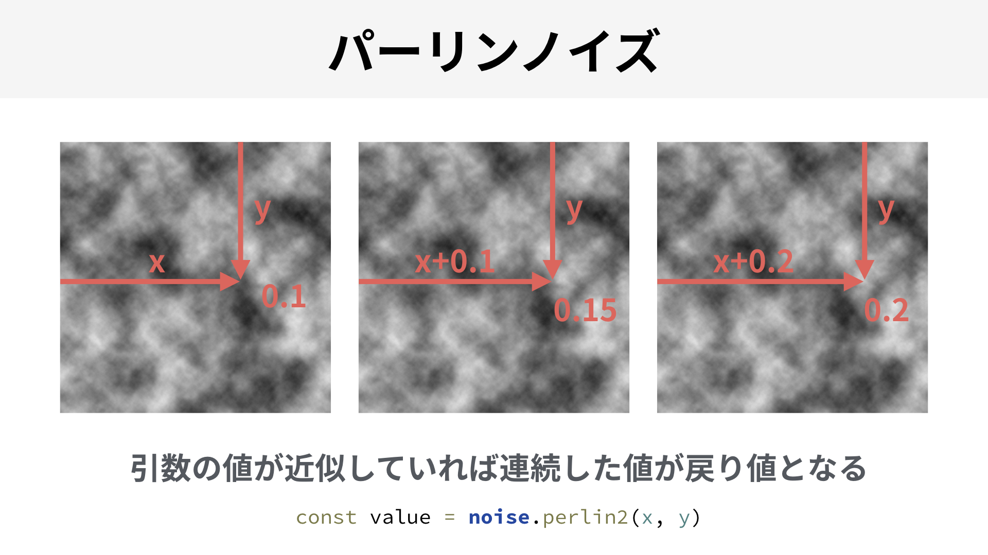
Using continuous noise makes it possible to create wave-like results, for example.

In the next demo, you can confirm that nearby input values produce nearby output values. Move the X and Y sliders slowly and watch how the result changes.
Perlin noise is useful for effects such as waves and wind. It has many applications, so it is a technique worth learning if you are interested in creative coding. For more detail, see the ICS MEDIA article “パーリンノイズを使いこなせ”.
Apply the values computed with Perlin noise to the starting positions in GSAP.
for (let i = 0; i < dots.length; i++) {
  const dot = dots[i];

  // Read the original index order that was stored at creation time.
  // This is used to reconstruct the particle's original position.
  const index = dot.offsetIndex;

  // Normalize the X position to a range from 0.0 to 1.0.
  // Particles near the left edge become closer to 0,
  // and particles near the right edge become closer to 1.
  const nx = (index % lengthW) / lengthW;

  // Normalize the Y position to a range from 0.0 to 1.0 as well.
  // Particles near the top edge become closer to 0,
  // and particles near the bottom edge become closer to 1.
  const ny = Math.floor(index / lengthW) / lengthH;

  // Feed the normalized coordinates into Perlin noise.
  // Nearby particles return similar values,
  // producing motion that feels random but continuous.
  const px = noise.perlin2(nx, ny);
  const py = noise.perlin2(nx * 2, ny);

  tl.from(
    dot,
    {
      // Scale the noise values by the stage size
      // and use them as the starting position.
      x: stageW * px,
      y: stageH * py,
      alpha: 0,
      duration: 4,
      ease: "expo.inOut",
    },
    // Start all particles together first
    // so the effect of the noise is easier to observe.
    0,
  );
}
The result bends and warps in an organic way.
Create a left-to-right flow
Next, make the particles appear as if they flow in from the left side of the screen. The idea is to incorporate the X coordinate into each tween’s delay.
// Particles on the left start earlier, and particles on the right start later.
// Because nx is already in the range from 0.0 to 1.0,
// it can be used directly as the delay.
const delay = nx * 1.0;

// (Some code omitted)

tl.from(
  dot,
  {
    x,
    y,
    alpha: 0,
    duration: 4,
    ease: "expo.inOut",
  },
  // By shifting the start time slightly for each particle,
  // the motion appears to flow from left to right.
  delay,
);

The entrance and exit of the particles now have a visible sense of flow.
Add a touch of randomness
If the coordinates computed from Perlin noise are used as-is, the pattern can feel too regular. Add one more layer of randomness to break it up.
// Slightly change the noise inputs
// so the X and Y directions move differently.
const px = noise.perlin2(nx, ny * 2);
const py = noise.perlin2(nx * 2, ny);

// Keep the left-to-right timing difference.
const delay = nx * 1;

// Scatter particles on the left more strongly.
// This helps reinforce the feeling that the text is flowing in.
const spread = (1 - nx) * 100 + 100;

// Noise alone can feel too orderly,
// so add random values at the end
// to create a more natural amount of variation.
const x = stageW * px + Math.random() * spread;
const y = stageH * py + Math.random() * spread;

tl.from(
  dot,
  {
    x,
    y,
    alpha: 0,
    duration: 4,
    ease: "expo.inOut",
  },
  // Apply both the flow from noise
  // and the flow created by time offsets.
  delay,
);

This reduces the overly orderly feel.
Final result
Finally, add the finishing touches. Different easing functions are used for the entrance and exit to shape the lingering feel of the motion, and an additional effect is added so the particles gradually move slightly toward the viewer.
That concludes the main tutorial. The rest is optional reading for anyone who wants to go deeper into the technical details.
Column: Rendering a large number of particles efficiently
Even with GPU rendering such as WebGPU, moving a large number of elements at once still requires paying attention to both CPU and GPU load. In general, reducing draw calls and cutting unnecessary CPU-side work are practical places to start when optimizing.
In this demo code, context.getImageData(0, 0, imageW, imageH) is called only once, and the resulting pixel array is reused, avoiding per-pixel calls to getImageData(). In addition, PIXI.Texture.from(image) creates a single shared texture, and each particle uses PIXI.Rectangle to crop only the region it needs.
All particles are then managed together inside a PIXI.Container, which makes it easy to control scaling and centering in one place. PixiJS also offers faster options such as ParticleContainer, but this implementation uses a regular Container because it needs flexible per-particle control over properties such as scaleX, scaleY, and alpha.
The basic ideas behind GPU rendering optimization have not changed since the WebGL era. If you want to learn more about draw-call optimization, see the article “WebGLのドローコール最適化手法”.
Column: Perlin noise and simplex noise
Perlin noise was developed by Ken Perlin. It was originally created for the 1982 film Tron. For many years, Perlin noise has been used in many contexts. For example, Adobe After Effects includes Fractal Noise and Turbulent Noise, and Adobe Flash’s BitmapData class had a perlinNoise() method that is, as the name suggests, Perlin noise itself.
In 2001, Perlin introduced simplex noise. Compared with Perlin noise, simplex noise requires less computation and runs faster. I debated whether to explain this article using Perlin noise or simplex noise, but I chose Perlin noise because it is more widely known. Their usage is not very different, after all.
The following 2021 article introduces the subtle differences in the values produced by Perlin noise and simplex noise. According to the article, simplex noise seems to have less bias.
I do not know how much impact that difference in tendency has on the final visual result, but anyone who can identify at a glance whether something was made with Perlin noise or simplex noise must have a remarkable eye.
As a side note, the article 神の書 Making Things Move! の続編、詳解ActionScript3.0アニメーション mentions that Keith Peters, who wrote about the difference between Perlin noise and simplex noise, is also the author of Foundation ActionScript 3 Animation, a book often regarded as a classic in the Flash community. Even now that Flash Player is gone, it is nice to see that the experts who worked deeply with Flash are still active.
Column: Why the text was prepared as an image
To keep things simple, the text was prepared as an image. Why use an image instead of drawing the text directly?
Canvas 2D has a fillText() method for drawing text. That approach would work, but if the generic sans-serif family is used, the actual font differs by environment, so the result is not consistent.
A possible solution would be to use web fonts. However, to use web fonts with Canvas 2D, the font needs to finish loading before drawing starts. Detecting whether the font has finished loading is not straightforward, and it may require a JS library such as WebFontLoader. For more detail, see the article “HTML5 CanvasとWebGLでウェブフォントを扱う方法”.
In other words, the code becomes far too complex for what this article is trying to do, so an image was used instead.
Bonus: Trying the same idea without WebGPU or JS libraries
As a bonus, I tried building a similar effect using div elements and the standard Web Animations API instead of WebGPU and JS libraries.
(It runs slowly, so open it in a new window.)
The runtime cost is high, so increasing the particle count much further seems difficult. The animation code is also messy. In my view, the Web Animations API is well suited to simple motion, but not to motion that combines multiple kinds of behavior.
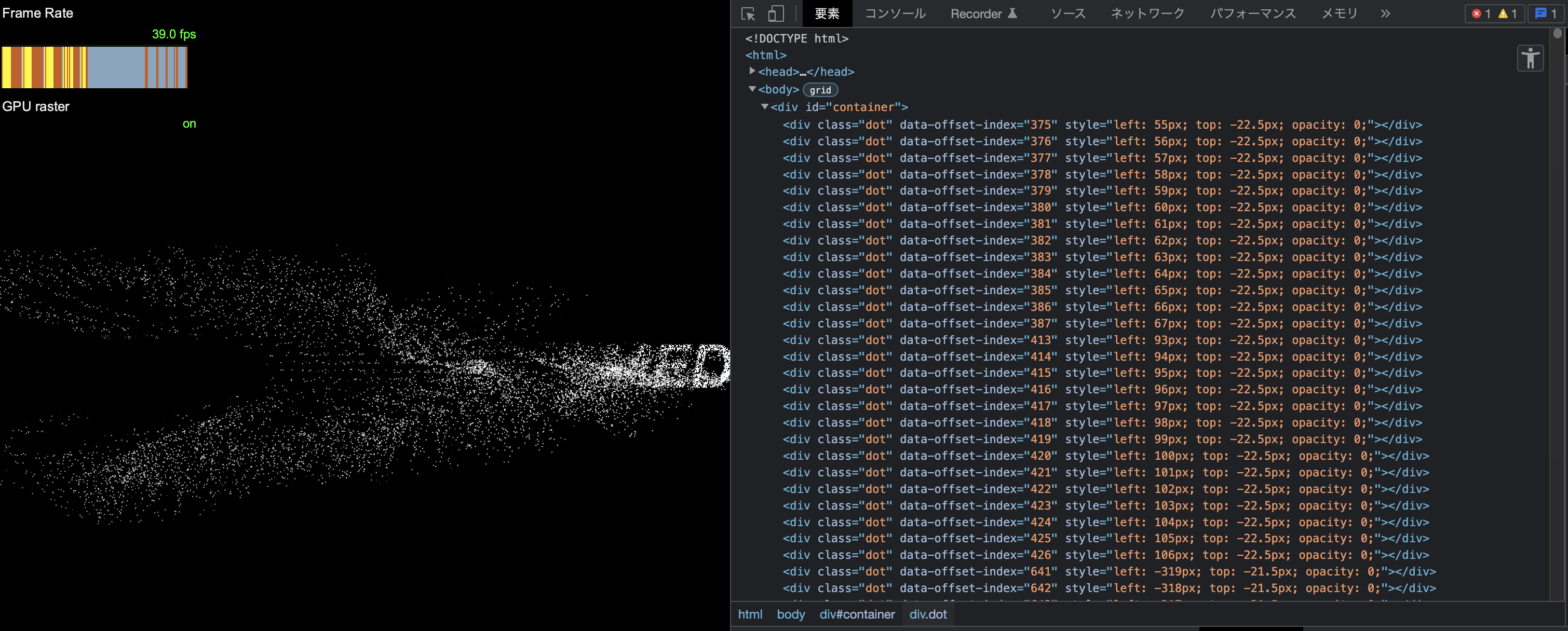
Rendering is faster with WebGPU, but when choosing a technology stack, it is important to build comparison demos and judge which approach is appropriate. I already had a good idea what would happen if I built it with the DOM, but producing actual evidence still matters.
Conclusion
The key point of this article is that motion can often be built by combining small techniques, and that it is fun to refine visual expression through experimentation. I hope this article encourages more people to explore creative coding.